Class 12 - Design I - (Quasi)-Experimental Data
Agenda
Quasi-experimental designs: what, why, when, how (30 minutes)
Application paper discussion (30 minutes)
Replication presentation (Group 15 minutes)
Skills corner - Class walkthrough in R (25 minutes)
General discussion (10 minutes)
Break then Class 13
Quasi-experimental designs
Preamble: Curve-fitting v. causality
Two different regimes:
Curve-fitting: Statistically identifying the parameters of a mathematical relationship between two or more variables based on the observed data, and making a law-like statement that summarizes empirical regularities
Causality: Imposing further structure to impose an if-then logical sequencing; where a change in one variable will necessarily have a causal impact on the other. Usually couched in terms of counterfactuals or “but for” reasoning: if not for the change in X, we would have observed a different Y
What is a “quasi-experiment”?
A quasi-experiment is a study that takes place in a field setting and involves a change in a key independent variable of interest but relaxes one or both of the defining criteria of laboratory and field experiments: random assignment to treatment conditions and controlled manipulation of the independent variable (Grant and Wall 2009, 655)
What is a “quasi-experiment”?
“Natural experiments” as a form of quasi-experiment:
Quasi-experiments also include changes to an independent variable that are naturally occurring rather than manipulated (Grant and Wall 2009, 655)
What is a “quasi-experiment”?
What about “regression discontinuity designs”?
Regression discontinuity designs (RDDs) are sometimes also called cutoff-based designs. They assign units to conditions based on a cut- off score on an ordered assignment variable, with units that fall on one side of the cutoff receiving treatment and those on the other side receiving the comparison condition. (Shadish and Cook 2009, 615)
What is a “quasi-experiment”?
What about “interrupted time series” or “structural breaks”?
Similar to RDD, an effect is measured as a change in the slope or intercept of the time series at the point of treatment introduction. (Shadish and Cook 2009, 617)
Why are quasi-experiemental designs useful?
Per Grant and Wall (2009), the benefits include but are not limited to:
strengthening causal inference when random assignment and controlled manipulation are not possible or ethical; and
building better theories of time and temporal progression.
Employing a quasi-experiement
What are the common threads among many of these designs?
Two groups: treatment and control
The amount of “randomness” differs across the designs
The distinction between treatment and control also varies
What are the common threads among many of these designs?
Two+ time periods or comparison points: pre-/post or with/without treatment
The period of followup before and after differs
The “fuzziness” of the treatment can also vary
What are the common threads among many of these designs?
Accounting for covariates
Random assignment is used to “wash out” differences between the groups
Propensity scores and control variables used to account for residual differences
The aim: The experimental ideal
Experimenter intervention in selection of indepedent variable (treatment)
Random assignment to treatment and control group
Creation of a stark counterfactual: what would happen but for the treatment?
Assuming complications like “compliance” and other experimental design concerns are addressed, this allows for a clean determination of counterfactuals
The aim: The experimental ideal
Per Rubin’s Potential Outcomes Framework (Angrist and Pischke 2008):
\[E[y_{1i}|d_i = 1] - E[y_{0i}|d_i = 0] =\] \[\pmb{E[y_{1i}-y_{0i}|d_i = 1]} + (E[y_{0i}|d_i = 1] - E[y_{0i}|d_i = 0])\]
The LHS (top) is the difference between the treatment and control group in the population
The bolded term is the “average treatment effect on the treated” - the causal effect that occurs for the treated group
The RHS term in parentheses is the selection bias
The aim: The experimental ideal
\[E[y_{1i}|d_i = 1] - E[y_{0i}|d_i = 0] =\] \[\pmb{E[y_{1i}-y_{0i}|d_i = 1]} + (E[y_{0i}|d_i = 1] - E[y_{0i}|d_i = 0])\]
The appeal of the experimental ideal is twofold:
We have a treatment and control group to estimate the LHS.
We use random assignment to set the selection bias term to 0.
Taken together, this allows us to identify the causal effect of interest.
How can you design a quasi-experiement?
A potential second-best option: Difference-in-differences
Perhaps we can’t get to the experimental ideal.
But let’s say we do have a treatment and a control group that have been selected via a “natural experiment” (e.g., close elections, change in regulations, exogenous shocks) that helps us mitigate selection bias.
We can track the change in outcomes over time for both groups and get a difference before the treatment \(t_1\) (pre-treatment) and after the time of treatment \(t_2\) (post-treatment).
We can then look at the difference-in-differences between these two groups to estimate the causal effect.
Estimating difference-in-differences
D-i-D as a comparison of means: \(DiD = (Y_{post,treated}-Y_{pre,treated})-(Y_{post,control}-Y_{pre,control})\)
D-i-D in a regression framework: \(Y = \beta_0+\beta_1T+\beta_2\delta+\beta_3\delta T\)
where \(\delta\) = 0 indicates pre-treatment and \(\delta\) = 1 indicates post-treatment and T = 1 indicates in the treatment group while T = 0 indicates the control group
In this setup, the estimated coefficient \(\beta_3\) is the D-i-D estimator
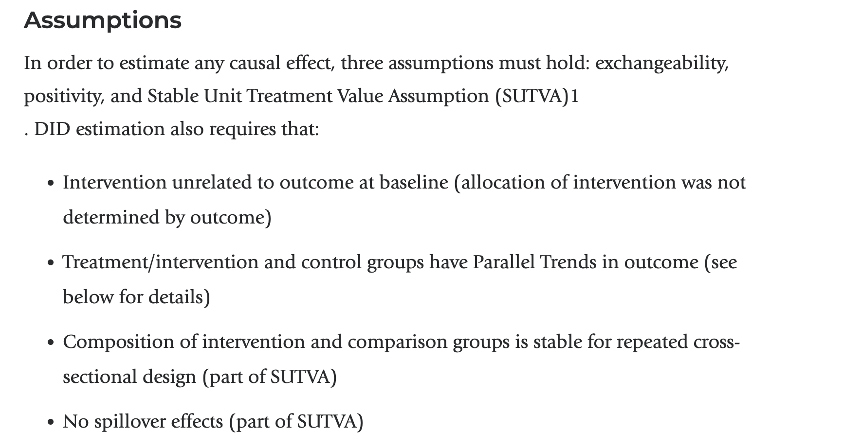
Assumptions
There are many assumptions to make the interpretation of a difference-in-differences casual:
Selected comparisons to difference-in-differences
RDD: Does not require temporal differences, identification of effect through discontinuity in a continuous variable that determines placement in treatment group
Structural breaks: Does not have a contemporaneous control group, the assumption is that the existing trend would continue but for the structural break
Randomized field experiments: Closer to experimental ideal in principle but can be logistically challenging and faces hurdles of attrition, incomplete treatment , and Hawthorne effects
Lab experiments (e.g.,Shu et al. (2012) and countless OB lab studies): Closer to experimental ideal but there could be significant issues with external validity / generalizability beyond the lab setting
Applications
Application readings
Let’s level-set people’s familiarity with these pieces.
Shu, L. L., Mazar, N., Gino, F., Ariely, D., & Bazerman, M. H. (2012). Signing at the beginning makes ethics salient and decreases dishonest self-reports in comparison to signing at the end. Proceedings of the National Academy of Sciences, 109(38), 15197–15200. doi:10.1073/pnas.1209746109 (see also https://datacolada.org/109)
Penrosian capacity as a constraint on entrepreneurial growth: An exploratory study employing the dot-com bubble (working paper)
Shu et al (2012)
What was this paper about?
What were the findings?
What was the method?
What makes sense? What was confusing?
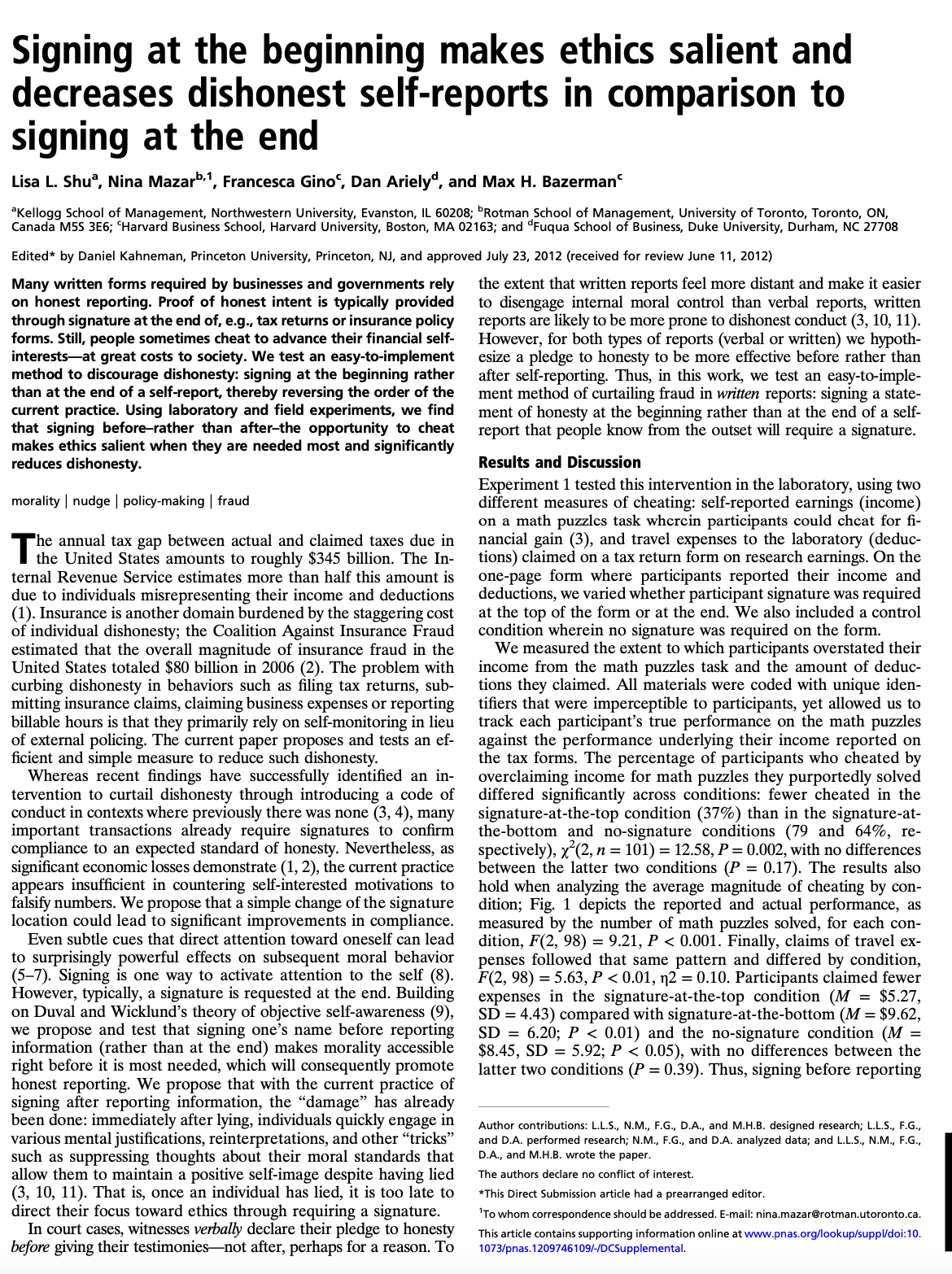
Did you notice anything funny about this paper?
It has been retracted.
Let’s see why and how the process unfolded
Yay science!
Yay science?
Another example from Economics
[ ]
]
Fox Souder and Johnson (working paper)
What was this paper about?
What were the findings?
What was the method?
What makes sense? What was confusing?
Break
Replication Presentation
- Replication: Penrosian capacity as a constraint on entrepreneurial growth: An exploratory study employing the dot-com bubble (working paper)
Skills corner - Class walkthrough in R
Preparation for next class
Next class
Design II: Longitudinal Data
Ployhart, R.E. and R.J. Vandenberg. 2010. Longitudinal Research: The Theory, Design and Analysis of Change. Journal of Management, 36(1): 94-120.
Mitchell, T. R. & James, L. R. 2001. Building better theory: Time and the specification of when things happen. Academy of Management Review, 26: 530-548.
Next class
Design II: Longitudinal Data
Applications:
Certo, S. T., Withers, M. C., & Semadeni, M. 2017. A tale of two effects: Using longitudinal data to compare within- and between-firm effects. Strategic Management Journal, 38(7), 1536-1556.
Replication: Firm Repertoires and Performance: The Influence of Complementarity and Competition (working paper)