
Class 7 - Elements IV: Measures and data

Agenda

  • Conceptual grounding (5 minutes)

  • Core paper discussion (25 minutes)

  • Final Compare-contrast presentation (30 minutes)

  • Break

  • Skills corner: Descriptive statistics (30 minutes)

  • First pass at Class 8 materials (30 minutes)

Grounding

Switching things up a bit

  • This class marks our transition from a research design to research methods focus

  • Thus, the order of presentation is a little fluid this class, with less emphasis on discussing the core papers at length

The rubber meets the road

  • Measures: Translating our variables into concrete measures (these do not need to be 1 to 1)

  • (Sourcing) Data: Where are we going to find these measures? [to be discussed in workshop]

Readings for Today

Common Readings

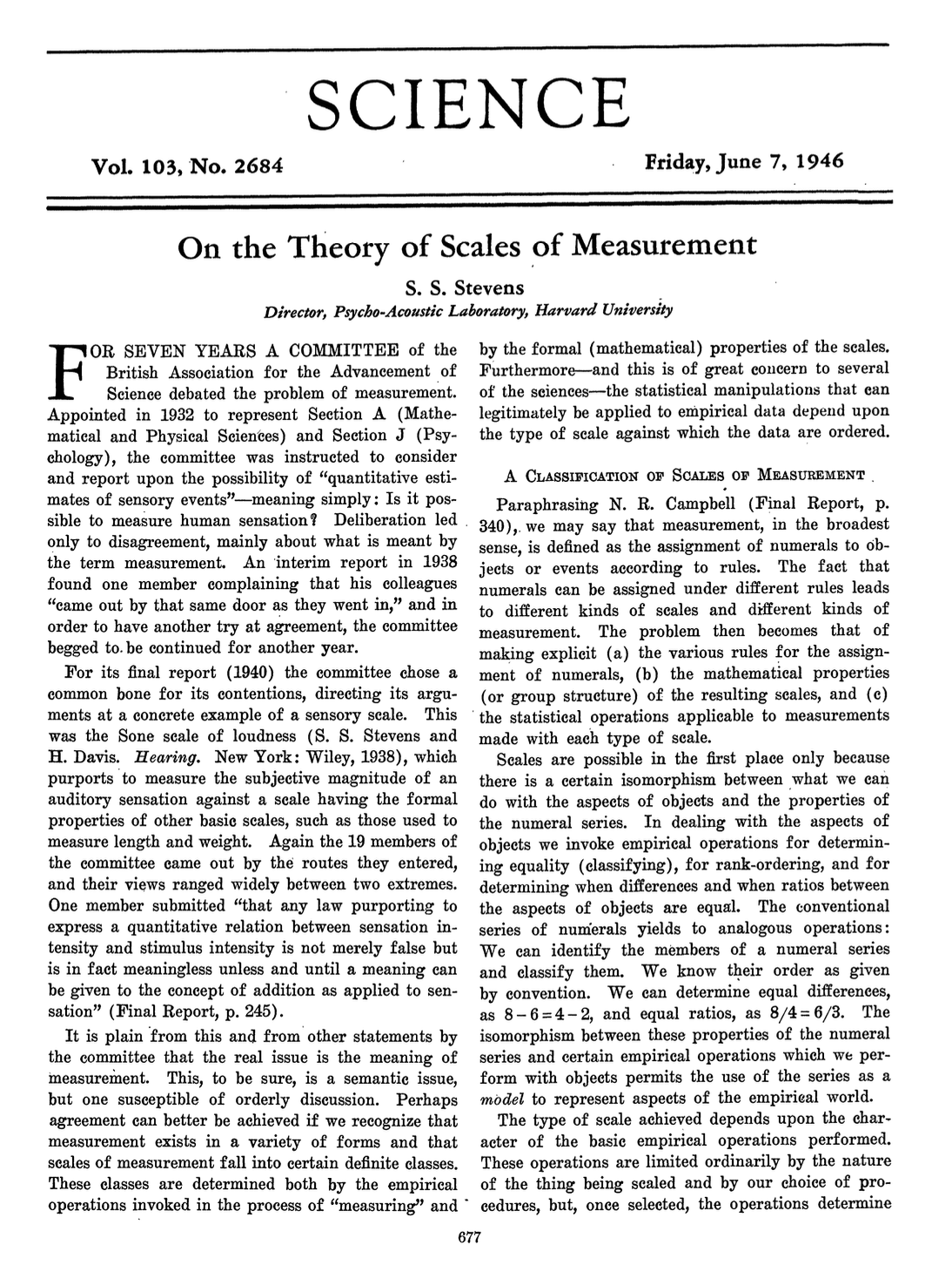
  1. Stevens, S. S. 1946. On the Theory of Scales of Measurement. Science, New Series, 103, No. 2684, 677-680.

  2. Bedian, A. G. 2014. “More Than Meets the Eye”: A Guide to Interpreting the Descriptive Statistics and Correlation Matrices Reported in Management Research. Academy of Management Learning & Education, 13, No. 1, 121-135.

  3. Heggestad, E. D., Scheaf, D. J., Banks, G. C., Monroe Hausfeld, M., Tonidandel, S., & Williams, E. B. (2019). Scale Adaptation in Organizational Science Research: A Review and Best-Practice Recommendations. Journal of Management, 45(6), 2596-2627.

Stevens (1946)

Paraphrasing N. R. Campbell (Final Report, p. 340),. we may say that measurement, in the broadest sense, is defined as the assignment of numerals to objects or events according to rules. The fact that numerals can be assigned under different rules leads to different kinds of scales and different kinds of measurement. (Stevens 1946, 677)

Stevens (1946)

Discussion Questions (briefly)

  • Are there types of measurements that are not discussed in this article?

  • What would happen if you make inferences about a measurement using the wrong type of scale?

Stevens (1946)

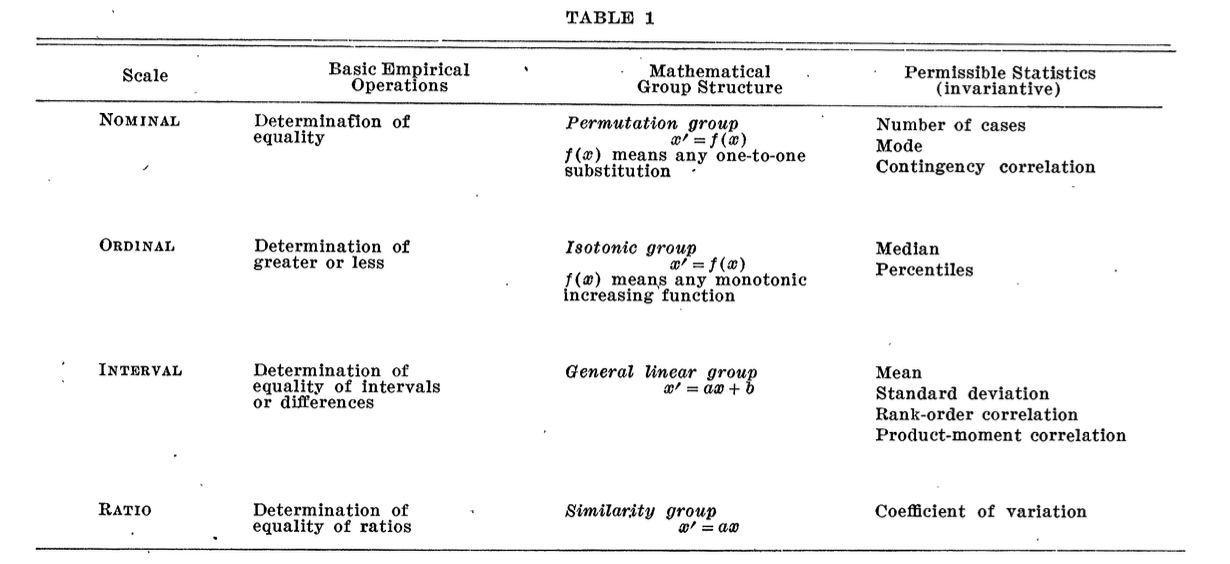
Basically, I grabbed this seminal paper to show where the different scales of measurement originated from: these are commonly referenced categories.

Heggestad et al (2019)

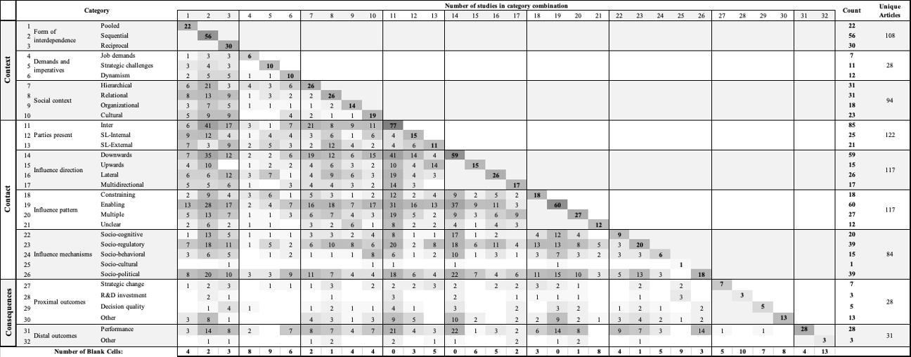
Heggestad et al (2019)

Discussion questions (briefly)

  • What is a scale, again?

  • Why would you want to change one that is already in the literature?

Heggestad et al (2019)

Key points

  • Scales are very common, particularly in micro research

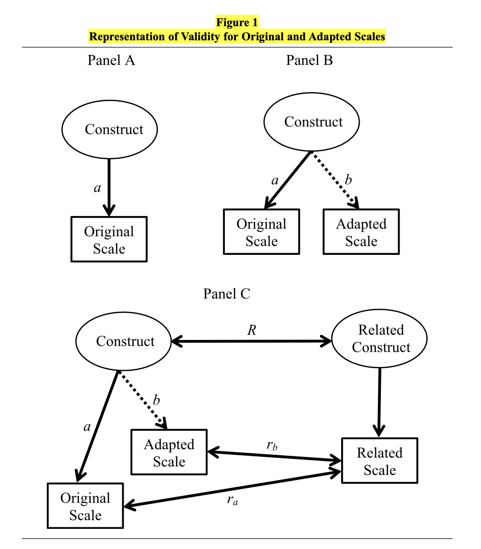
  • They are a common basis to establish construct validity

  • They are an example of where data and variables are not 1 to 1, and thus adaptations are possible

  • While I would argue some of this concern is a bit overblown, the point is conceded that material changes to a scale may unmoor it from its validated basis

Bedian (2014)

Discussion Questions (briefly)

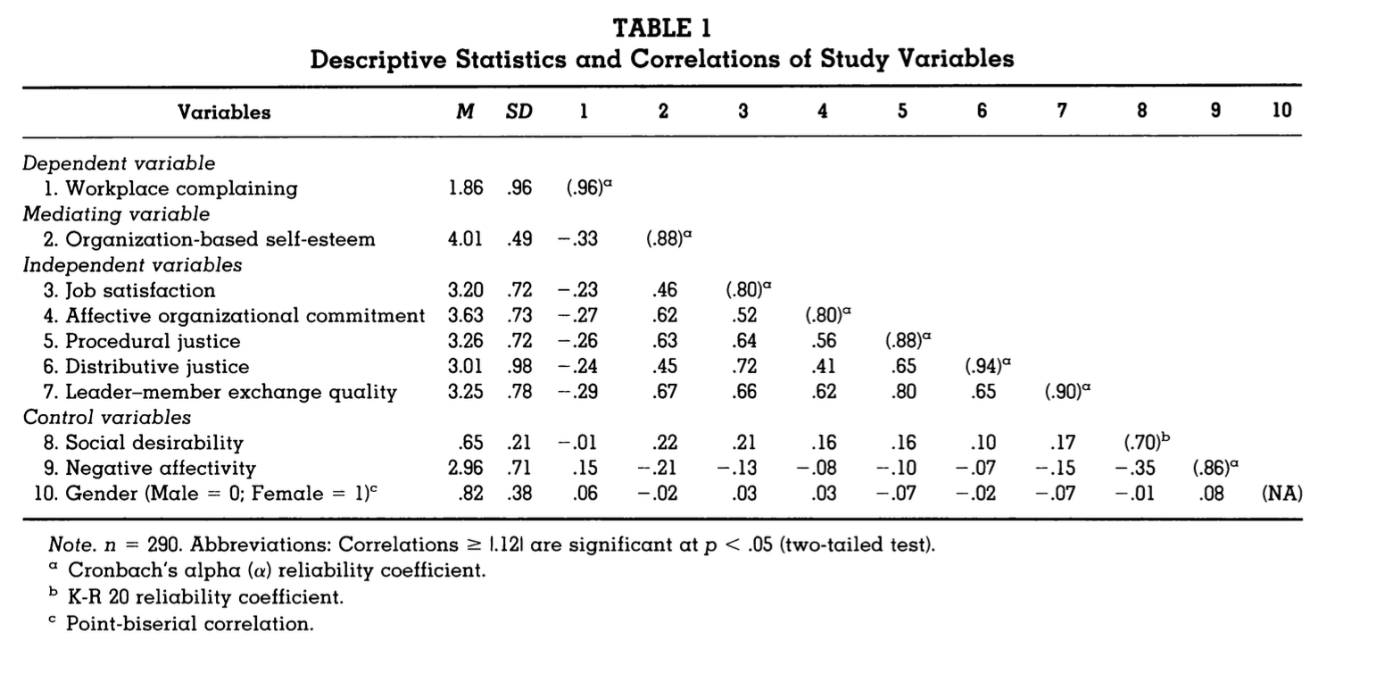
  • Did you know you could extract so much information from a single table?

  • While this is a nice list of ‘sanity checks’, is this really all that descriptive statistics can tell us? [more to come in a bit on this point]

Bedian (2014)

The 12-point checklist

  1. Disclosed Mean, SD, Correlations
  2. Sensible frequency distributions
  3. Feasible standard deviations
  4. Reported reliabilities (multi-item scales)
  5. Feasible correlations
  6. Wonky looking scatterplots

Bedian (2014)

The 12-point checklist

  1. Accounted for common data collection methods
  2. “Correct” signs (see also Kennedy (2008))
  3. Assessment of collinearity (e.g., VIFs)
  4. Sensible “point-biserial” (e.g., binary) correlations?
  5. Disclosed data missingness
  6. Disclosed sampling procedure

Readings for Today II

Compare / Contrast Presentations

  • Combs, J. G. 2010. Big samples and small effects: Let’s not trade relevance and rigor for power. Academy of Management Journal, 53(1): 9-13.

  • Simsek, Z., Vaara, E., Parachuri, S., Nadkarni, S., & Shaw, J. D. 2019. New ways of seeing big data. Academy of Management Journal, 62: 971-978.

Break

Skills corner

The power of descriptives

Quick reminder:

  • Descriptive statistics: Procedures for depicting the main aspects of sample data, without necessarily inferring to a larger population

  • Inferential statistics: Techniques that allow inferences about characteristics of a population to be drawn from a sample of data from that population

The power of descriptives

Descriptive statistics help you understand and tell the story of your data and the sample it is drawn from

Inferential statistics provide you the means to generalize that story beyond your sample given certain assumptions (often, but not always, by appealing to a parametric model)

Essentials: Distributions and summary statistics

Probability distribution: A mathematical description of a random phenomenon in terms of its sample space and the probabilities of events (subsets of the sample space)

Many of the properties of a distribution can be summarized by its moments:

  • Mean or expected value

  • Variance (or deviations from the mean)

But other descriptives are often very informative, such as interquartile range (IQR), range (Max - Min), and others.

Example 1: A normal distribution

── Attaching core tidyverse packages ──────────────────────── tidyverse 2.0.0 ──
✔ dplyr     1.1.4     ✔ readr     2.1.5
✔ forcats   1.0.0     ✔ stringr   1.5.1
✔ lubridate 1.9.4     ✔ tibble    3.2.1
✔ purrr     1.0.4     ✔ tidyr     1.3.1
── Conflicts ────────────────────────────────────────── tidyverse_conflicts() ──
✖ dplyr::filter() masks stats::filter()
✖ dplyr::lag()    masks stats::lag()
ℹ Use the conflicted package (<http://conflicted.r-lib.org/>) to force all conflicts to become errors
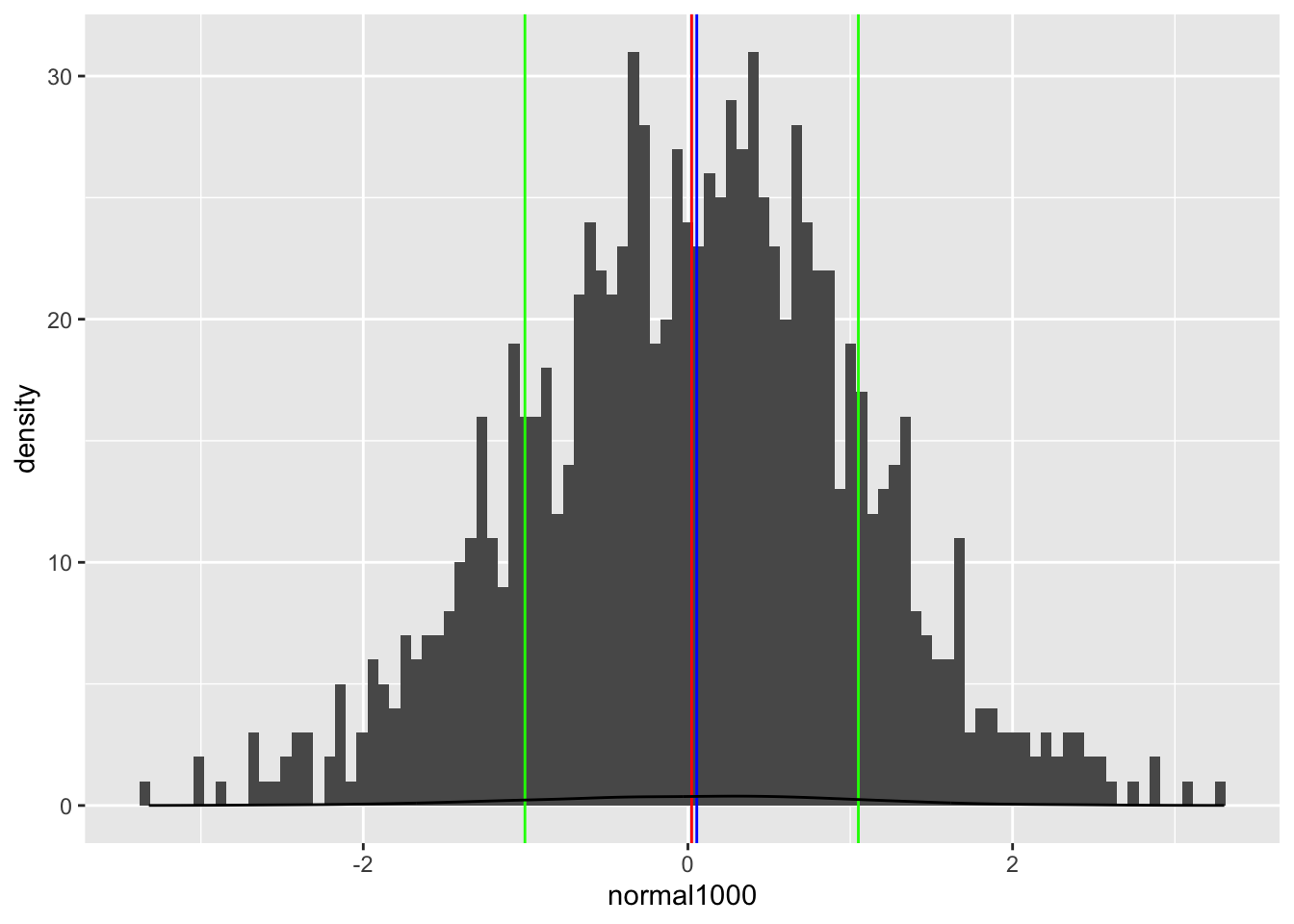
Figure 1: A normal distribution

Note the mean (red), median (blue), and standard deviations (green). A normal distribution can be completely summarized by its mean and variance.

Example 2: A log-normal distribution

Figure 2: A log-normal distribution

By contrast, in this distribution the mean and median diverge, and the standard deviations are wonky - more information is required to characterize this distribution.

Essentials: Distributions and summary statistics

Note how the summary statistics distill key features without seeing the whole thing.

paste("Normal Distribution")
[1] "Normal Distribution"
summary(normal)
    Min.  1st Qu.   Median     Mean  3rd Qu.     Max. 
-3.32078 -0.64316  0.05468  0.02295  0.70855  3.30415 
paste("SD:", round(sd(normal),3))
[1] "SD: 1.027"
paste("Log-Normal Distribution")
[1] "Log-Normal Distribution"
summary(lognormal)
    Min.  1st Qu.   Median     Mean  3rd Qu.     Max. 
 0.03612  0.52563  1.05620  1.71767  2.03104 27.22542 
paste("SD:", round(sd(lognormal),3))
[1] "SD: 2.267"

Essentials: Univariate visualizations

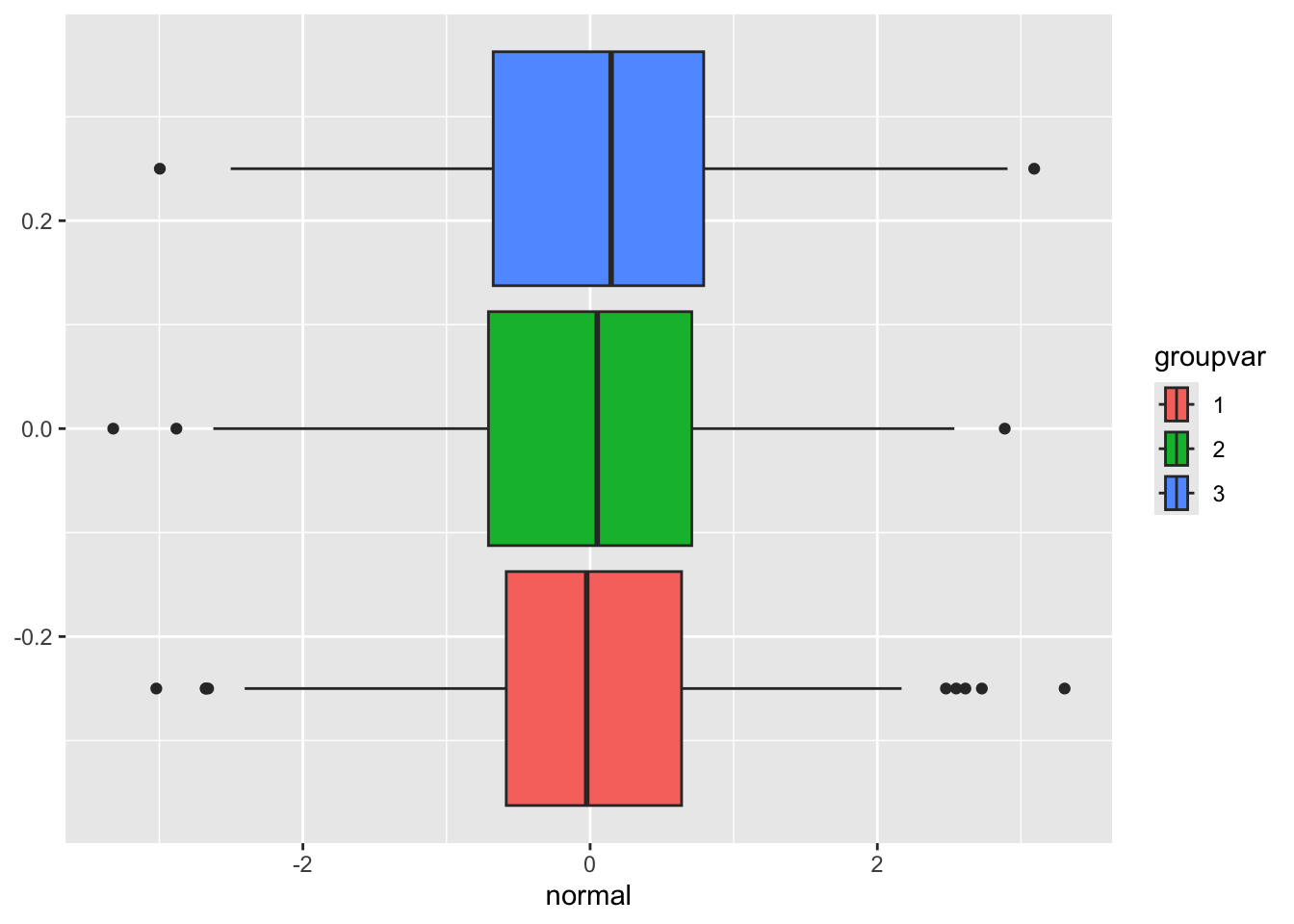
Histograms (shown above) are very useful, but other tools like boxplots can be just as helpful to identify issues, such as outliers.

ggplot(data=distributions,aes(x=normal,fill=groupvar))+geom_boxplot()

Essentials: Correlation matrices

When we move to multiple variables, correlation matrices take center stage, often complemented by scatterplots (Bedian 2014).

Essentials: Scatterplots and trendlines

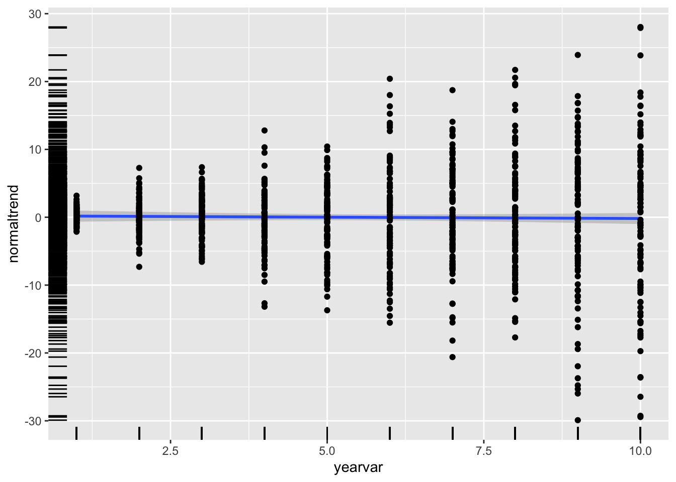
Here is an example multi-graph, with “marginal” rug plot, scatterplot, and linear trend.

ggplot(data=distributions,aes(x=yearvar,y=normaltrend))+geom_rug()+geom_smooth(method="lm", se=T)+geom_point()
`geom_smooth()` using formula = 'y ~ x'

Catching issues

Doing a thorough review of your data through a descriptive lens can help identify issues that will turn up in your analysis, such as:

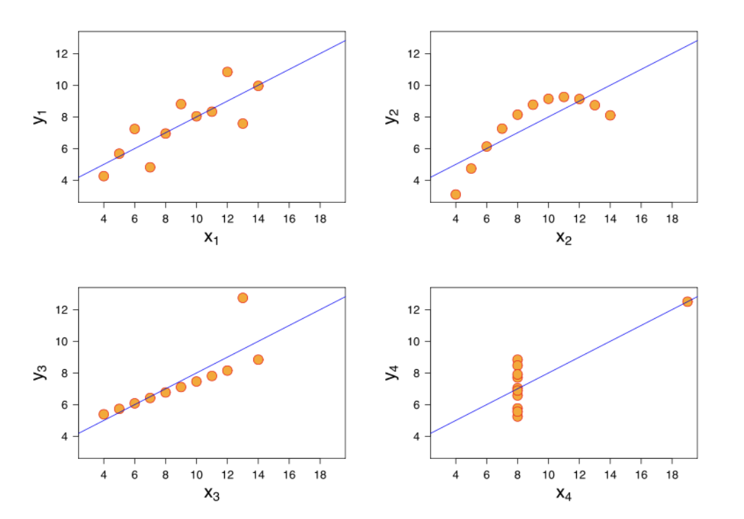
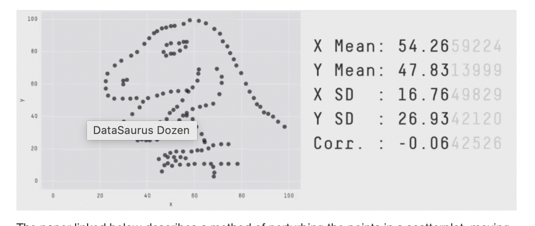
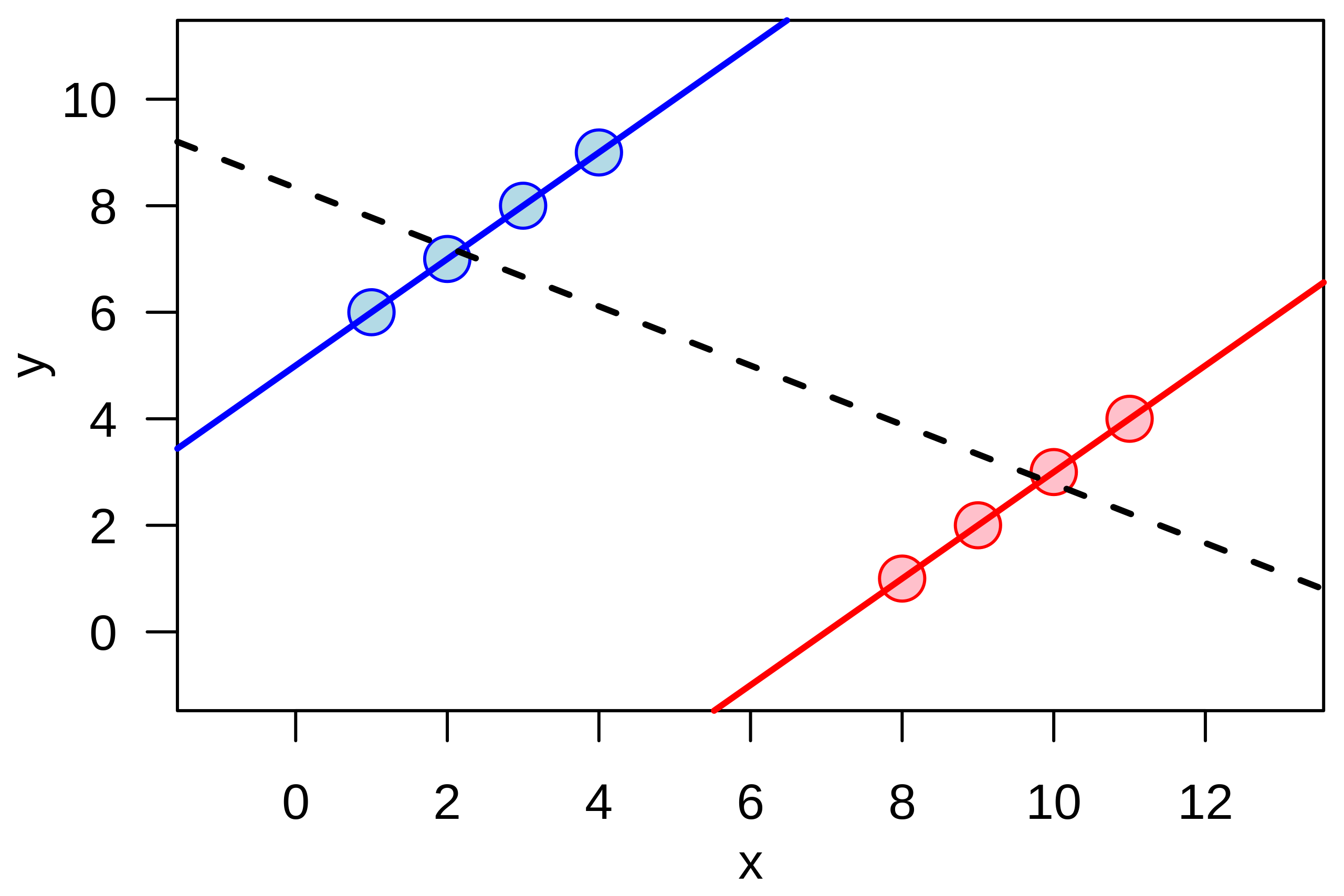
  • Deceptive descriptives - a.k.a. the datasaurus dozen

  • Range restriction or selection issues - no data for certain conditions

  • Non-linearity - potential cut-off or non-linear effects

  • Heteroskedasticity - uneven variances across the distribution or group-level effects

  • Outliers - influential observations that throw off a trendline (n.b.: when are outliers noise and when are they the signal?)

Catching issues: Anscombe’s quartet

Anscombes’ Quartet

The Datasaurus Dozen

Catching issues: Simpson’s paradox

Simpson’s Paradox

Telling stories with data

Beyond being a prelude to inferential analyses, descriptives can also help to tell your story directly

  • Cross-tabulations (i.e., 2x2s)

  • Group comparisons (e.g., pre- / post- intervention)

  • “Existence proofs” (presence and/or variation of a construct)

Telling stories: Cross-tabulations

Cross-tab example

Telling stories: Group comparisons

Showing, not telling the results of a regression discontinuity design

Preview of next class

From descriptives to inference

  • As we just covered, descriptive statistics can be very powerful, but often we want to move from the sample to the population.

  • In other words, we seek to make broader inferences

  • There are many ways to do this, but a common workhorse is regression, which will serve as the backbond of the next several weeks

Recall: The paradigm of our class

This class is rooted in a paradigm

  • We have a well-articulated research question (Classes 1-3)

  • We will build a model with hypotheses to answer this question (Classes 4-7)

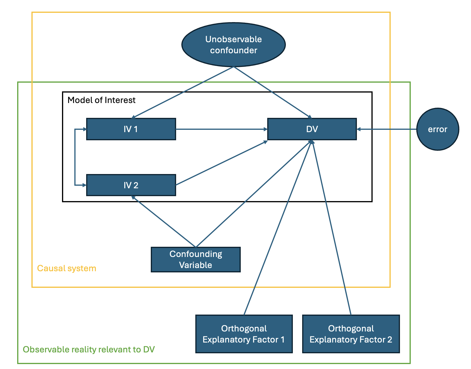
  • That model is nested within a causal system and reality

  • Our hope is to recover a causal effect through an estimation process (Classes 8-12)

For this to be effective, we want this estimate to be:

  • Accurate: hopefully unbiased, but at least consistent

  • Precise: “efficient”, using sample information well

How your model fits within this paradigm

On the following slide, I illustrate how your focal model compares to the wider system of relationships

  • Note that you may need to include elements outside of your model of interest to specify the causal system (Class 5: Models + Hypotheses)

  • Also note that our model may be influenced by observable and unobservable factors (Class 6: Constructs + Variables)

  • This presumes you have a story you want to understand rather than trying to maximize the predictability of the DV (a different question to answer)


Let’s take a quick preview of Class 8 now

Next class

Techniques I: Regression

  1. Kennedy, P. 2008. A Guide to Econometrics (6th Edition ed.). Malden, MA: Blackwell. [Chs. 3 and 4]

  2. Carlson, K. D., & Wu, J. 2012. The illusion of statistical control: Control variable practice in management.

Next class

Techniques I: Regression

Applications:

  1. Replication: Simsek, Z., Fox, B., & Heavey, C. 2021. Systematicity in Organizational Research Literature Reviews: A Framework and Assessment. Organizational Research Methods, 109442812110086.

  2. Katila, R., & Ahuja, G. 2002. Something Old, Something New: A Longitudinal Study of Search Behavior and New Product Introduction. Academy of Management Journal, 45(6), 1183-1194.

How it will work

Everyone should read the first two articles in detail, they provide grounding

Everyone should have a working familiarity with the application papers (what the study is about, how the tests were performed, key findings)

One group will actively try to replicate the findings with data and code that I provide and report out the process

Workshop

Objectives

We have two objectives with our workshop today:

  1. Share your updated research questions and models

  2. Expose you to two tools that may help perform your empirical work

    • WRDS: a goldmine of organizational level data
    • RStudio: a powerful envirionment to perform statistical analyses

Given the way the time breaks down, we will do 2. and then 1.

Workshop Agenda

  • Pulse Check

  • Sourcing data (11-12p)

    • Generally
    • Worked example with WRDS and R
  • Research Model Presentations (1-4p)

  • Reflections

Class Pulse Check

Pollev.com/drfox

Sourcing data

  • Given the variation in your interests and topics, it is not productive to talk at length about data sourcing since it is unique to your circumstances (but we will walk through one example)

  • But here are some ideas on the following two slides

Sourcing data - Primary sources

Collecting specifically what you need for a study

  • Field surveys

  • Experiments (lab or field) with purpose-built collection instruments

  • Interviews / focus groups

  • Direct observation / ethnographic methods

Sourcing data - Secondary sources

Relying upon others to collect data or using ‘unobtrusive’ measures

  • Archival datasets (e.g., Factiva, COMPUSTAT, Biocentury, SDC)

  • Publicly available survey data (e.g., Kauffman Firm Survey, Census ACS)

  • Industry reports (e.g., Wohler’s Reports)

  • Video, audio, or written artifacts (CEO speeches, earnings calls, 10-Ks, website scraping)

  • Company records

  • Cliometric methods (historical archives)

Example: Sourcing and analyzing data using WRDS and R

  • WRDS
    • A commonly employed data source for business search, containing hundreds of databases
    • Not all are accessable, the licenses are institution dependent
    • Many mentioned above accessed here (e.g., CRSP, Compustat, BoardEx)
  • R Studio
    • A powerful statistical software environment that allows you to analyze, visualize, and report empirical data and results

Protocol

  1. Set-up RStudio and test it is working
  2. Set-up WRDS
  3. Get some data from WRDS
  4. Run some basic commands in RStudio

RStudio Setup

  • Install R: https://cran.rstudio.com/
  • Install R Studio: https://posit.co/download/rstudio-desktop/
  • Load up R Studio and walk through the environment using “Elementary R References” in Dropbox
    • Principles of Econometrics in R (pp. 9-12)
    • R for Data Science (Ch. 1)
  • Quick tour of the “mpg” dataset using ggplot (for generating graphics)

Getting new data: WRDS

Examining the data with RStudio

  1. Save your CRSP data to the desktop with name “crspdata.txt”
  2. Go to R Studio
  3. Open the “Class 7 Example” file I have provided in Dropbox
  4. Let’s work from there

Questions before switching gears?

Research Presentations

Reflections

References

References

Bedian, Arthur G. 2014. “‘More Than Meets the Eye’: A Guide to Interpreting the Descriptive Statistics and Correlation Matrices Reported in Management Research.” Academy of Management Learning &Amp; Education 13, No. 1: 121–35.
Kennedy, Peter. 2008. A Guide to Econometrics. Malden, MA: Blackwell.
Stevens, S. S. 1946. “On the Theory of Scales of Measurement.” Science New Series, 103, No. 2684: 677–80.