Class 8 - Techniques I - Regression

Agenda

The logic of regression: what, why, when, how (40 minutes)
Application paper discussion (20 minutes)
Break
Replication presentation (15 minutes)
Skills corner - Class walkthrough in R (25 minutes)
General discussion (15 minutes)

The logic of regression

Preamble

I will weave in the “core” papers as needed in my remarks later, but we will not discuss them in detail per se

WARNING: I am going deeper into the weeds this week, but we will come back up to a higher level soon

What is a regression?

The multiple linear regression model is used to study the relationship between a dependent variable (\(y\)) and one or more independent variables (\(X\)). The generic form of the linear regression model is (Greene 2012):

\[\pmb y = \pmb X\pmb\beta + \pmb\epsilon\]

where \(\beta\) is computed as follows:

\[(\pmb X^T\pmb X)^{-1}(\pmb X^T\pmb y)=\pmb \beta\]

Let’s figure out why…

What is a beta coefficient?

Small aside: Note that in a “simple” (bivariate) regression with just one predictor and an intercept

\[y = \beta_0+\beta_1x + \epsilon\]

this funky formula is essentially:

\[Cov(x,y)/Var(x)=\beta_1\]

Note that in the multiple regression case, the same logic applies but to covariances and variances that have been “residualized” by accounting for all of the other X variables in the equation (Angrist and Pischke 2008)

What’s with the name “regression”?

“Galton observed that extreme characteristics (e.g., height) in parents are not passed on completely to their offspring. Rather, the characteristics in the offspring regress toward a mediocre point (a point which has since been identified as the mean)” (Wikipedia)

What do we usually mean when we say “regression”?

The term “regression” is often used synonomously with a particular technique: ordinary least squares (OLS).

Essentially, OLS and its generalizations (e.g., WLS, GLS, discussed later) seek to minimize the distance between observed and predicted values
It is constrained in this task in that only the data provided by X can be used, and that there are too many observations to simply interpolate

What is OLS doing?

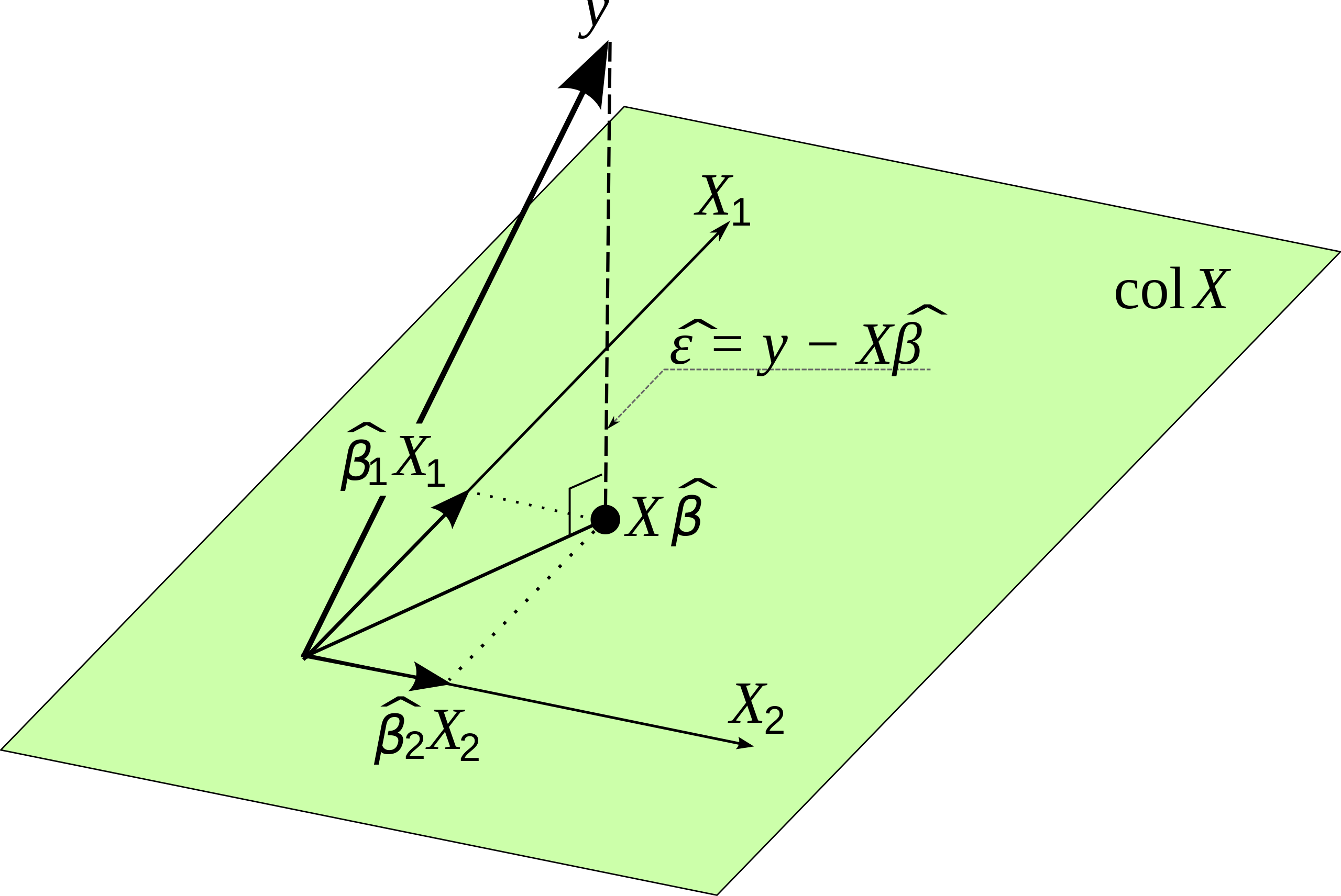
The data in X forms a (hyper)-plane, and each X variable is weighted by \(\beta\), resulting in a prediction
The discrepancy between this predicted value \(X\beta\) and \(y\) is the error term \(\epsilon\), which by definition is unrelated to the X variables

A sample data generating process

Let’s say we know that the relationship between X and Y is as follows:

\[y = (\beta_0=0)+(\beta_1=2)x + \epsilon\]

and that \(\epsilon\) is randomly distributed with mean of 0 and a standard deviation of 3.

This is an example data generating process, what might such data look like?

A sample data generating process

library(ggplot2)
library(tidyverse)

── Attaching core tidyverse packages ──────────────────────── tidyverse 2.0.0 ──
✔ dplyr     1.1.4     ✔ readr     2.1.5
✔ forcats   1.0.0     ✔ stringr   1.5.1
✔ lubridate 1.9.4     ✔ tibble    3.2.1
✔ purrr     1.0.4     ✔ tidyr     1.3.1
── Conflicts ────────────────────────────────────────── tidyverse_conflicts() ──
✖ dplyr::filter() masks stats::filter()
✖ dplyr::lag()    masks stats::lag()
ℹ Use the conflicted package (<http://conflicted.r-lib.org/>) to force all conflicts to become errors

set.seed(4352)

x = rep(seq(1:7),7)
y = 2*x + 3*rnorm(49,0,1)
data = as_tibble(cbind(x,y))


data[1:10,]

# A tibble: 10 × 2
       x      y
   <dbl>  <dbl>
 1     1 -0.714
 2     2  7.28 
 3     3  3.00 
 4     4  6.05 
 5     5 10.6  
 6     6 10.2  
 7     7 13.4  
 8     1 -2.31 
 9     2  3.78 
10     3  7.14

OLS as a mathematical procedure

The population regression equation applies to each observation (thus the matrix form):

\[\pmb y = \pmb X \pmb \beta + \pmb \epsilon\]

and beta is selected / defined to minimize the sum of the squared errors (i.e., positive and negative errors don’t cancel out):

\[min(\pmb \epsilon^T\pmb \epsilon) = (\pmb y - \pmb X \pmb \beta )^T(\pmb y - \pmb X \pmb \beta ) \]

In other words, we ask; what value of beta should we select to minimize the LHS?

OLS as a mathematical procedure

This minimization problem (with respect to beta) leads to the “normal equations” <- clink on the link for a full derivation.

\[(\pmb X^T\pmb X)^{-1}(\pmb X^T\pmb y)=\pmb \beta\]

Comments:

What would happen the if error/disturbance term was always zero?
Notice, this equation is agnostic to the form / distribution of the errors

OLS as an “estimator”

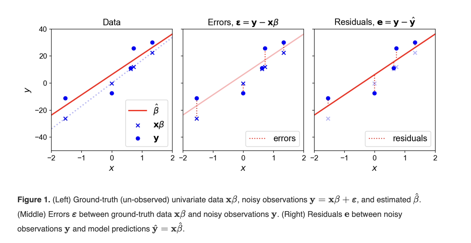
Remember, we don’t have the whole population, we just have a sample. Thus, the residuals we get from an OLS estimation are different from the underlying errors in the population due to sampling error in our estimate of \(\beta\)

OLS as an “estimator”

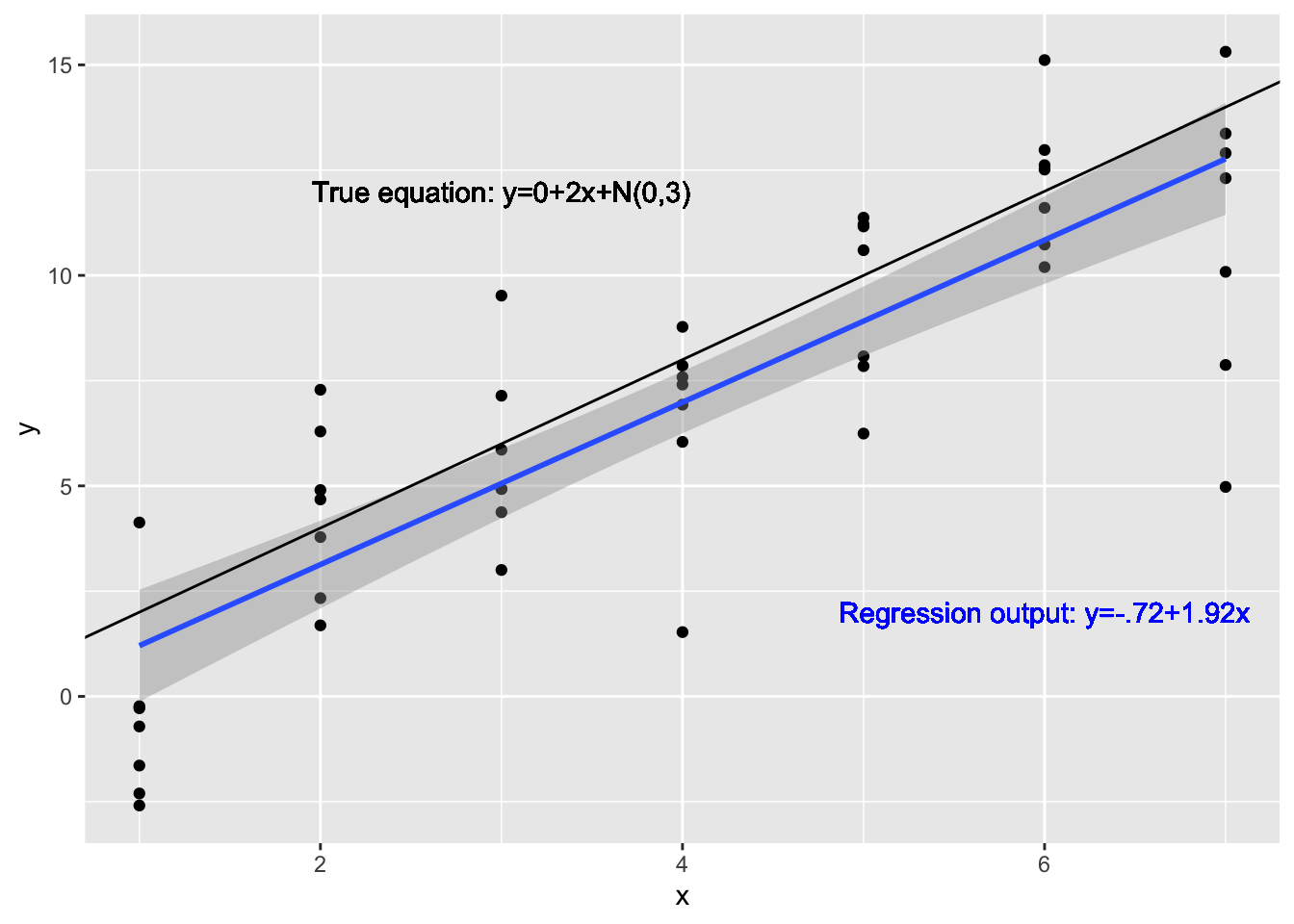
Here is another example of this distinction with the data we generated earlier. Recall the “true” parameters: \(y = (\beta_0=0)+(\beta_1=2)x + \epsilon\)

coef(summary(lm(y~x)))

              Estimate Std. Error    t value     Pr(>|t|)
(Intercept) -0.7233802  0.8190561 -0.8831876 3.816302e-01
x            1.9272462  0.1831465 10.5229748 6.023326e-14

OLS - Estimation v. reality

ggplot(data,aes(x,y))+geom_point()+geom_smooth(method='lm',se=T)+geom_text(x=6,y=2,label = "Regression output: y=-.72+1.92x",color="blue")+
  geom_text(x=3,y=12,label = "True equation: y=0+2x+N(0,3)") + 
  geom_abline(aes(intercept = 0, slope = 2))

`geom_smooth()` using formula = 'y ~ x'

Verifying our beta coefficient formula

Let’s verify that our simple equation for \(\hat b\) works out:

\[\hat Cov(x,y)/\hat Var(x)=\hat b_1\]

paste("cov(x,y)", cov(x,y))

[1] "cov(x,y) 7.8695885474943"

paste("var(x)", var(x))

[1] "var(x) 4.08333333333333"

paste("beta-hat", cov(x,y)/var(x))

[1] "beta-hat 1.92724617489656"

What is a regression? - Prediction versus explanation

Notice a few things:

OLS regression on a sample, by construction, minimizes the sum of the squared residuals
This means that it seeks to maximize the amount explained by the regression to maximize the chances of correctly predicting the data in the sample
By implication, it is NOT trying to find some true value of \(\beta\) such that we can make good out of sample predictions; issues with the sample will contaminate beta
It also does NOT imply an causal interpretation or explanation

Why linear regression and OLS in particular?

OK, then why are regressions ubiquitous?

Approximates the conditional expectation function (Angrist and Pischke 2008)
The “best linear unbiased estimator” or BLUE, when the Gauss-Markov assumptions met (Kennedy 2008)
Equivalent to maximum likelihood estimator (MLE) and maximum a posteriori estimator (MAP) when errors normally distributed (Kennedy (2008), p. 43) and with a uniform prior

Let’s consider each in turn.

“Approximates the conditional expectation function”

Recall that much of the information we want to extract from a distribution is summarized in its first two moments: mean and variance

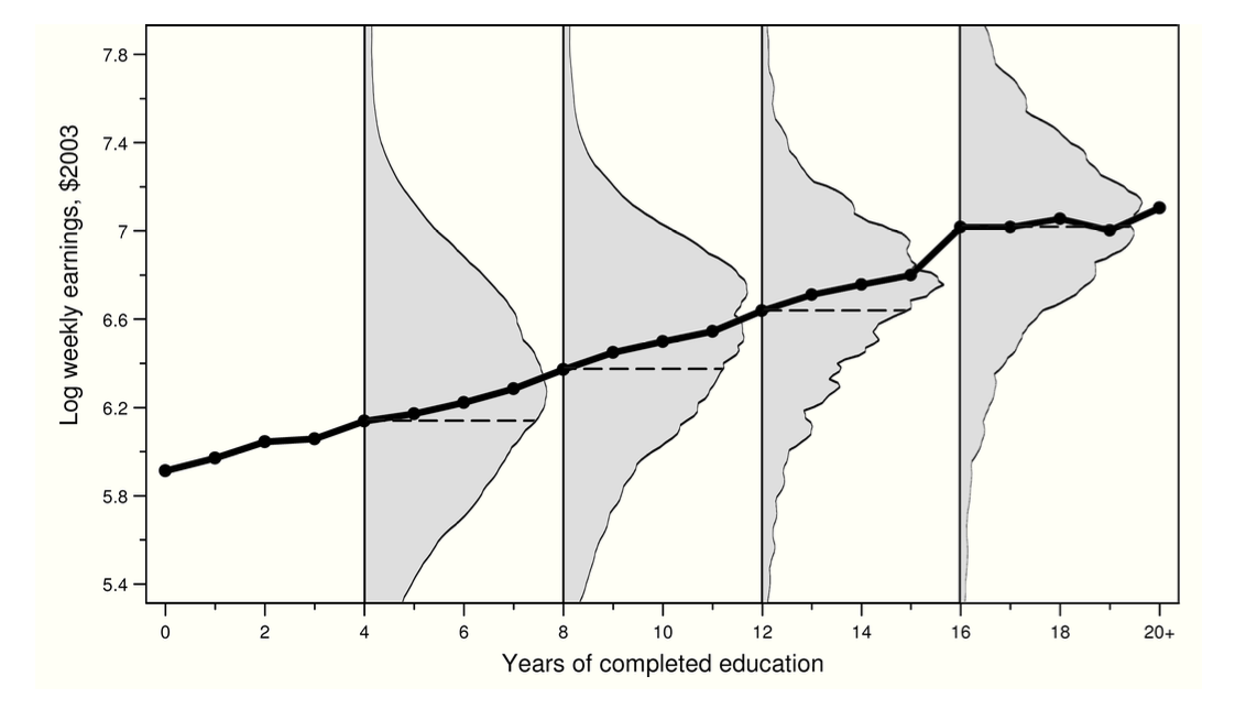
The conditional expectation function [CEF] expresses the expected value (or mean) of a variable (Y) as a function of another variable (X)

The CEF is often not linear, but the OLS estimator is the best linear approximation to the CEF function (Angrist and Pischke 2008, Theorem 3.1.6)

“Approximates the conditional expectation function”

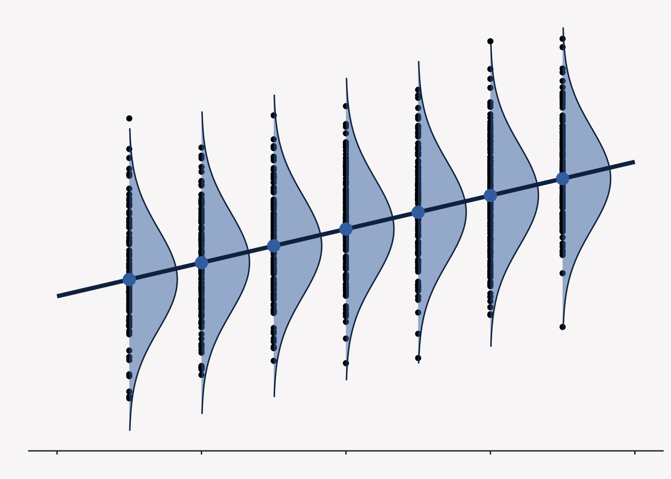
Note what this picture is showing you - it highlights the fact that Y has a distribution at each level of X, and what OLS can do is determine how that distribution “shifts” as you change X

“Approximates the conditional expectation function”

The “standard”, unmodified form of OLS assumes that the distribution of Y remains the same across all levels of X (i.e., the distribution is homoskedastic or possesses “spherical errors”), and that the only difference is a shift in where the mean is placed

#' scaled_dnorm
#' 
#' 
scaled_dnorm <- function(x, mean = 0, sd = 1, scale) dnorm(x, mean, sd) * scale

#' geom_norm_density
#' 
#' 
geom_norm_density <- function(mean, sd, fun, args, y_offset, color, fill,
                              alpha, scale) {
  ggplot2::geom_area(
    stat = "function",
    fun = fun,
    args = list(mean = mean, sd = sd, scale = scale),
    xlim = c(mean - 3 * sd, mean + 3 * sd),
    position = ggplot2::position_nudge(y = y_offset),
    color = color,
    fill = fill,
    alpha = alpha
  )
}

plot_alpha <- .50
plot_fill <- "#3F72AF"
plot_color <- "#112D4E"
plot_xlim <- c(-18, 18)

n <- 1000
x <- sample(1:7, n, replace = TRUE)
b <- 1
var_xb <- var(x*b)
std_error <- 9
y <- 2 + b*x  + rnorm(n, sd = sqrt(std_error))

data <- 
  tibble::tibble(
    x = x,
    y = y
  ) |>
  dplyr::mutate(
    y_cond_mean = 2 + x
  )

ggplot2::ggplot(
  data = data,
  ggplot2::aes(x = y, y = x)
) + 
  ggplot2::geom_point() + 
  geom_norm_density(
    mean = 3,
    sd = sqrt(9),
    scale = 5,
    fun = scaled_dnorm,
    y_offset = 1,
    color = plot_color,
    fill = plot_fill,
    alpha = plot_alpha
  ) +
  geom_norm_density(
    mean = 4,
    sd = sqrt(9),
    scale = 5,
    fun = scaled_dnorm,
    y_offset = 2,
    color = plot_color,
    fill = plot_fill,
    alpha = plot_alpha
  ) +
  geom_norm_density(
    mean = 5,
    sd = sqrt(9),
    scale = 5,
    fun = scaled_dnorm,
    y_offset = 3,
    color = plot_color,
    fill = plot_fill,
    alpha = plot_alpha
  ) +
  geom_norm_density(
    mean = 6,
    sd = sqrt(9),
    scale = 5,
    fun = scaled_dnorm,
    y_offset = 4,
    color = plot_color,
    fill = plot_fill,
    alpha = plot_alpha
  ) +
  geom_norm_density(
    mean = 7,
    sd = sqrt(9),
    scale = 5,
    fun = scaled_dnorm,
    y_offset = 5,
    color = plot_color,
    fill = plot_fill,
    alpha = plot_alpha
  ) +
  geom_norm_density(
    mean = 8,
    sd = sqrt(9),
    scale = 5,
    fun = scaled_dnorm,
    y_offset = 6,
    color = plot_color,
    fill = plot_fill,
    alpha = plot_alpha
  ) +
  geom_norm_density(
    mean = 9,
    sd = sqrt(9),
    scale = 5,
    fun = scaled_dnorm,
    y_offset = 7,
    color = plot_color,
    fill = plot_fill,
    alpha = plot_alpha
  ) +
  ggplot2::coord_flip() + 
  ggplot2::geom_line(
    data = data.frame(x = 0:8, y = 2 + 0:8),
    color = plot_color,
    lwd = 1.5
  ) + 
  ggplot2::geom_point(
    data = data.frame(x = 1:7, y = 2 + 1:7),
    size = 4,
    shape = "circle",
    group = 1,
    color = plot_fill,
    fill = plot_color
  ) +
  ggplot2::theme(
    plot.background = element_rect(fill = "#F9F7F7", colour = "#F9F7F7"),
    panel.background = element_rect(fill = "#F9F7F7"),
    axis.line.x = element_line(colour = "#3D3C42"),
    axis.line.y = ggplot2::element_blank(),
    panel.grid.minor = element_line(colour = "#F9F7F7"),
    panel.grid.major = element_line(colour = "#F9F7F7"),
    axis.ticks.y = ggplot2::element_line(linewidth = 0),
    axis.text.y = ggplot2::element_blank(),
    axis.text.x = ggplot2::element_blank()
  ) + 
  ggplot2::labs(
    x = "",
    y = ""
  )

“Best linear unbiased estimator” (BLUE)

If the Gauss-Markov assumptions are satisfied, then OLS is the:

Best (minimum variance among alternative estimators)
Linear(the estimator is of the form \(A(X)y\))
Unbiased (the expected value is equal to the population parameter)
Estimator (employs data from a sample to make inferences about the population)

Recent research seems to suggest that it might actually be the best unbiased estimator if these assumptions hold

“Equivalent to MLE and MAP under certain conditions”

There are other modeling frameworks to help make sense of data.

Maximum likelihood estimation or MLE: What parameter values make the data most likely, GIVEN an assumed distribution?
Maximum a posteriori (Bayesian) or MAP estimation: MLE that explicitly incorporates prior beliefs
Generalized method of moments: A “generalization” of MLE that focuses on moments rather than distributions

Note that MLE and GMM are the primary alternatives in our field to OLS/WLS/GLS: they are used for SEM, HLM, panel data estimators, logit, probit, and other models

“Equivalent to MLE and MAP under certain conditions”

When we have a uniform prior (all parameter values within an interval are equally likely) and when the error term is normally distributed, OLS provides the same estimate as MLE and MAP.

This should be somewhat comforting, since it implies:

The OLS estimate b is the most likely value for \(\beta\), given the data and assuming the distribution is normal
The OLS estimate is what we should update our beliefs to be if we did not have an informative prior

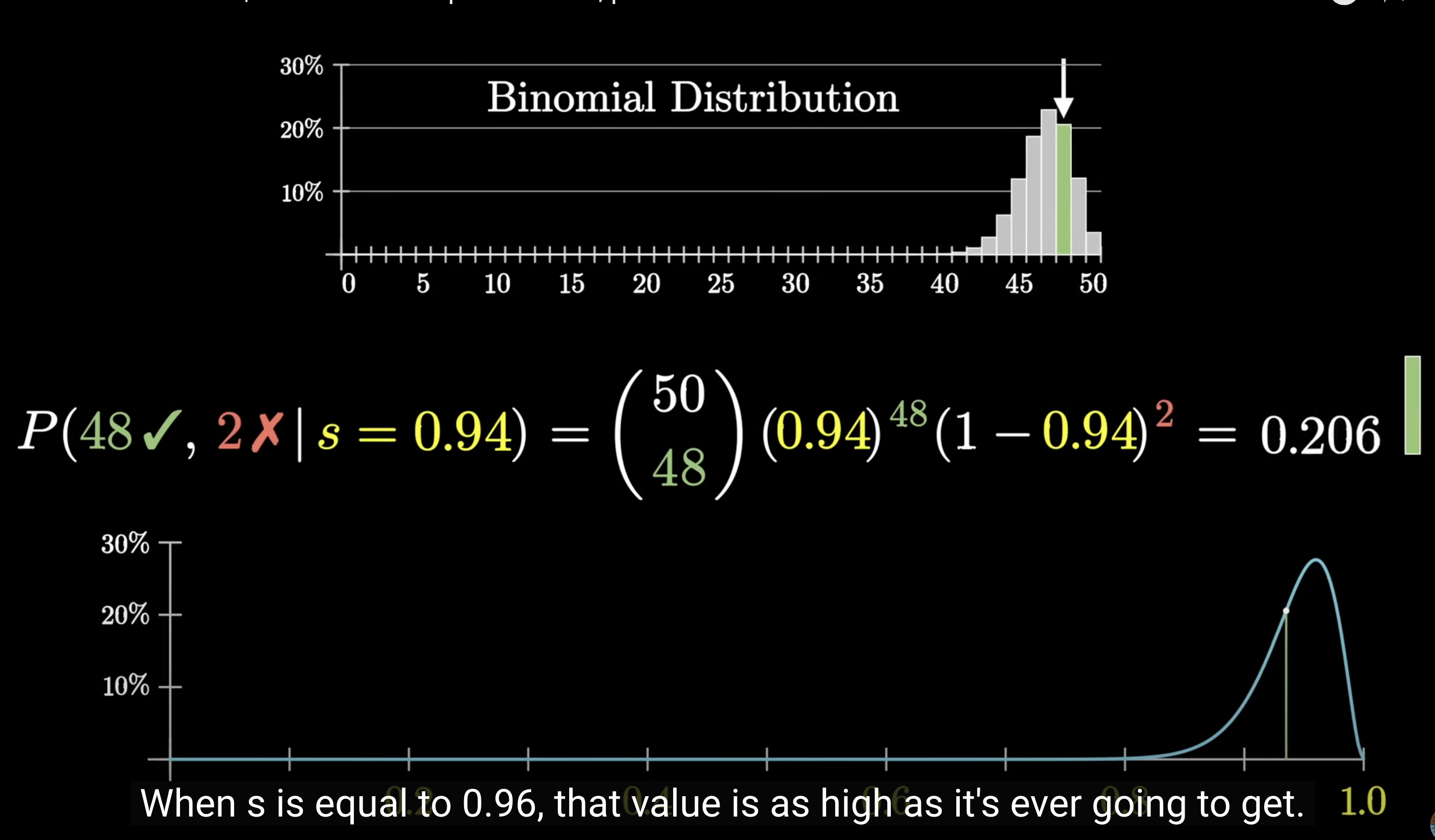
Aside: An example of how likelihood functions work

When is linear regression appropriate and / or optimal?

When the assumptions are satisfied!

And what are those assumptions? There are two “flavors”:

Fixed design
Random design

I’ve tried to align the numbering so that they correspond, where possible.

When is linear regression appropriate and / or optimal?

When is linear regression appropriate and / or optimal?

“Random design”

Linearity (model is correctly specified)
Spherical errors \(V[\pmb \epsilon|\pmb X] = \sigma^2\pmb I\)

implies: Homoskedaticity \(V[\epsilon|\pmb X] = \sigma^2\)
implies: No serial correlation \(V[\epsilon_i\epsilon_j|\pmb X] = 0; i \ne j\)

Strict exogeneity \(E[\epsilon|\pmb X] = 0\)
No multicollinearity (X is invertible)
Normality (optional) - allows us to make inferences about the sampling distribution of b

When is linear regression appropriate and / or optimal?

The Gauss-Markov theorem proves that, given these assumptions, the OLS estimator is the BLUE

It becomes the best unbiased estimator if normality is assumed (it reaches the Cramer-Rao lower bound)
The assumption of a spherical errors can be relaxed via Aitken’s theorem, known as weighted (WLS) or generalized (GLS) least squares
GLS often performs a transformation of the raw data to take into consideration the variance structure

Aside: alternative estimators when OLS/GLS not applicable

Maximum likelihood estimation (MLE)
Bayesian / maximum a posteriori (MAP) techniques
Generalized method of moments (GMM) estimators
Quantile regression
Machine learning (e.g.,random forest models)
LASSO (least absolute shrinkage and selection operation)
Markov Chain Monte Carlo simulation and bootstrapping
K-L divergence based metrics (e.g., Expectation-Maximization algorithms)

Performing a regression analysis

How to properly perform a regression analysis?

We determine the appropriateness of regression for our model and data from two angles:

Column (variable) perspective
Row (observation) perspective

Once we are satisfied that there are no issues (or that they have been addressed), run a “final, publication ready” regression.
Interpret the results using the tools of statistical inference (discussed later today).

The column (variable) perspective

Conditional mean structure

Do we have the right variables? (DAGs, theory)
Is the model in the correct functional form specified? (RESET,Chow tests)
Are the variables exogenous? (Sargen-Hansen, Durbin-Wu-Hausman)
Are your models well-conditioned? (VIF)

Variance structure

Is the mean structure correct? (see above)
Tests of heteroskedasticity and auto-correlation (e.g., Durbin-Watson, White tests)

The row (observation) perspective

Conditional mean structure

Are there outliers present? (Cook’s distance)
Are there influential observations? (hat matrix)
Are certain observations missing or partially missing? (Censoring and truncation
Is the model dynamic in nature? (Arellano-Bond estimators)

Variance structure

Is there a nested structure to the data? (Level of analysis)

Deep dive: Do we have the right variables?

Note that we don’t really have a “test” to apply here, but the assumption of proper specification is critical (including the right variables)

Why? Because if it is violated we don’t only lose the “best” part of BLUE, we also lose the “unbiased” part, and then we are just “LE”

And furthermore, the estimator isn’t even “consistent” -> i.e., gets closer to the true value as we increase the size of the sample, which is a “fall-back” position we can take if we don’t have an unbiased estimator for smaller samples

The issue: Omitted variable bias

Omitted variable bias causes ALL of the beta estimates in a model to be biased in proportion the correlation between the regressors and the omitted variable left in the error term

This bias can be expressed in terms of “short” and “long” regression estimates, where short means a relevant variable \(b_2\) has been omitted and the long is where it has been included (and it is assumed that the error term is truly uncorrelated in the case of the long equation):

In the simple case, the upshot is the short regression coefficient \(b_1\) will be biased in the following manner:

\[b_{1short} = b_{1long} + b_{2omitted}(cov(b_1,b_2)/var(b_1))\]

The issue: Omitted variable bias

The problem: remember that OLS assumes by construction that the error term and the X variables are uncorrelated, so we can’t rely on a quick test of their correlation to draw conclusions. You need to know from theory or experience that you are missing the variable and then can run the test of including it to see if it changes the results (assuming it is something you can measure!)

What can you do if this variable is unobservable? [See our endogeneity day!]

The flip side: The “illusion of statistical control”

By mapping practices to these purposes, we demonstrate why current CV practice struggles to accomplish any of them effectively while potentially reducing the interpretability of results. Empirically, we examine correlations between CVs and independent variables (IVs)—relationships that receive little consideration in standard CV practice—demonstrating these relationships can and do influence the magnitude and sign of regression coefficients, sometimes dramatically—just not very often. In fact, the CVs in the studies we reviewed most often have little if any impact on research find- ings or interpretations, creating the illusion of statistical control when little control actually occurs. (Carlson and Wu 2012, 415)

What if we fail to meet one or more of the assumptions?

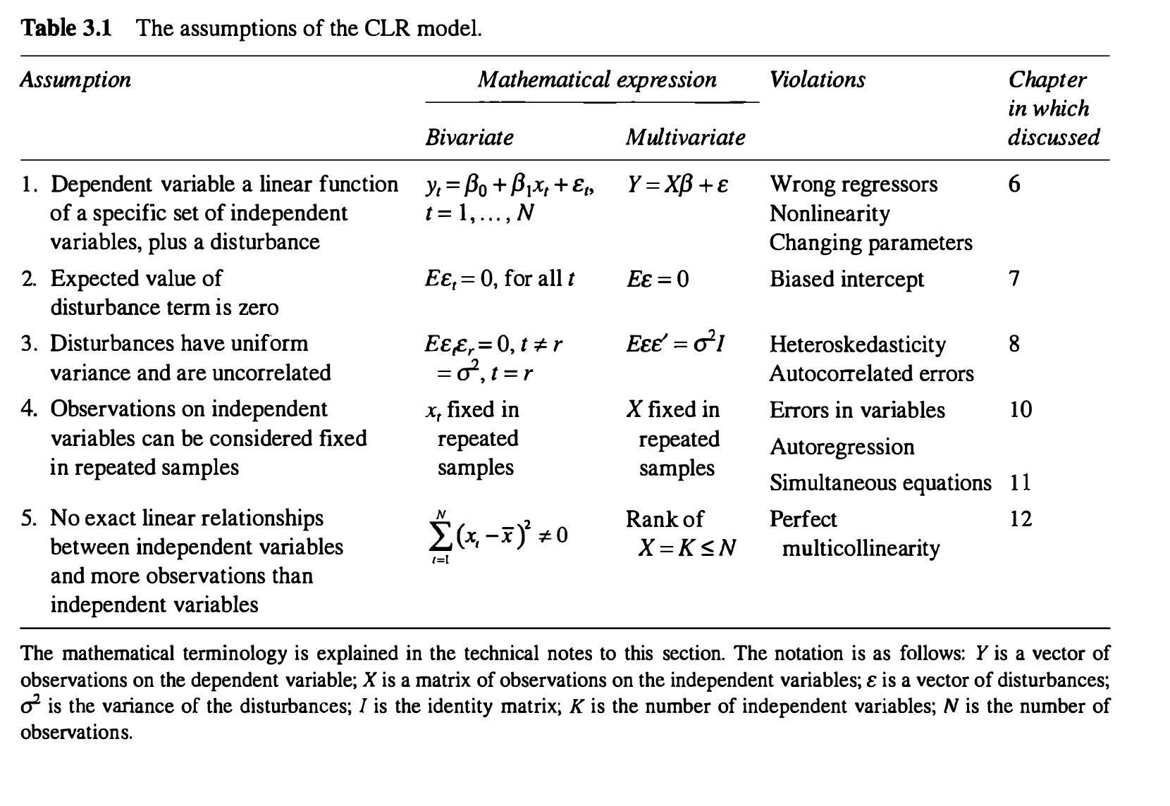
An econometrics textbook can be characterized as a catalog of which estimators are most desirable in what estimating situations. Thus, a researcher facing a particular estimating problem simply turns to the catalog to determine which estimator is most appropriate for him or her to employ in that situation. The purpose of this chapter is to explain how this catalog is structured. (Kennedy 2008, 40)

What if we fail to meet one or more of the assumptions?

But note that:

If more than one of the CLR model assumptions is violated at the same time, econometricians often find themselves in trouble because their catalogs usually tell them what to do if only one of the CLR model assumptions is violated. Much recent econometric research examines situations in which two assumptions of the CLR model are violated simultaneously. These situations will be discussed when appropriate. (Kennedy 2008, 44)

Statistical inference

Are our results “statistically significant”?

Once we have an estimate for \(\beta\) (known as \(\hat b\)), here are two approaches to statistical inference (Kennedy 2008):

Explicitly assume that the error term is distributed normally (t-tests and F-tests are appropriate straight away, even for small samples)
Rely on the central limit theorem and large-N asymptotics (beta is an expected value, so its distribution will convergence to a normal distribution - see this video to understand why)

The distribution of \(\hat b\)

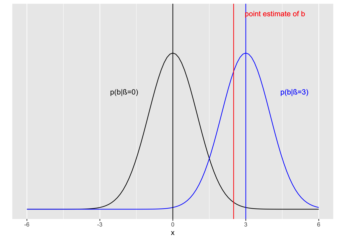
When making an inference, we ask where our point estimate (what we got from the regression) sits within the distribution of the estimator conditional on some assumed true value of \(\beta\)

library(ggplot2)

p1 <- ggplot(data = data.frame(x = c(-6, 6)), aes(x)) +
  stat_function(fun = dnorm, n = 101, args = list(mean = 0, sd = 1)) + ylab("") +
  stat_function(fun = dnorm, n = 101, color="blue", args = list(mean = 3, sd = 1)) + ylab("") + scale_y_continuous(breaks = NULL) +
    geom_vline(xintercept=0) +
      geom_vline(xintercept=3, color="blue") +
  geom_text(aes(x = -2, y = .3, label = "p(b|ß=0)"), stat = "unique") +
  geom_text(aes(x = 5, y = .3, label = "p(b|ß=3)"), color="blue") +
  geom_vline(xintercept=2.5, color="red") +
  geom_text(aes(x = 4.2, y = .5, label = "point estimate of b"), color="red")


  p1

Warning in geom_text(aes(x = -2, y = 0.3, label = "p(b|ß=0)"), stat = "unique"): All aesthetics have length 1, but the data has 2 rows.
ℹ Please consider using `annotate()` or provide this layer with data containing
  a single row.

Warning in geom_text(aes(x = 5, y = 0.3, label = "p(b|ß=3)"), color = "blue"): All aesthetics have length 1, but the data has 2 rows.
ℹ Please consider using `annotate()` or provide this layer with data containing
  a single row.

Warning in geom_text(aes(x = 4.2, y = 0.5, label = "point estimate of b"), : All aesthetics have length 1, but the data has 2 rows.
ℹ Please consider using `annotate()` or provide this layer with data containing
  a single row.

Determining appropriate standard errors

Questions about the variance structure also need to be settled:

Are errors spherical?
If not, do you want to incorporate the error structure information into the estimates (using GLS) or use OLS and “robust” statistics”?
Two schools of thought: Feasible GLS has no guarantees of improvement, but “Simply computing a robust covariance matrix for an otherwise inconsistent estimator does not give it redemption” (Greene 2012, 692)

Another word about “robust standard errors”

Per Angrist and Pischke (2008), pp. 40-48 - robust standard errors are computed using the method of moments, and justified asymptotically by the law of large numbers / central limit theorem (regardless of the underlying distribution of the estimator) Thus, the results are consistent regardless of the covariance structure but you need to worry about finite-sample bias

Statistical inferences you can draw

The simplest test:

Is \(\beta \ne 0\)?: Use t-tests

Intuition: We assume a null distribution that \(\beta = 0\), and then see where our estimated value falls within that distribution. The more extreme it is, the more likely the assumption that \(\beta = 0\) is false

Statistical inferences you can draw

A more powerful set of tests: linear hypotheses

Is \(\beta_1 = \beta_2\)?
Is \(\beta_1 = - \beta_2 + 2\beta_3\)?
Is \(\beta_1 = \beta_2 = \beta_3 = 0\)?

A restriction matrix is constructed to run an F-test (Wald test), Likelihood Ratio (LR) or LaGrange Multiplier (LM) test (Kennedy 2008, ch. 4)

Intuition: Unconstrained optimization (remember we are minimizing least squares) is easier than constrained. We ask whether there is a significant difference in model fit after imposing the restriction: If yes, then the restriction is probably false.

Examples:

“Linear hypothesis tests fail to reject the assertion that growth and reductions in either team size (\(\chi^2\)(1) = 0.39, p > 0.10) or within- industry experiences (\(\chi^2\)(1) = 0.17, p > 0.10) have equal and opposite effects” (Fox, Simsek, and Heavey 2023, 17)

“A Wald test indicates that the hypothesis that both variables are simultaneously zero is rejected (\(\chi^2\)(2) = 7.50, p = .02)” (Fox, Simsek, and Heavey 2022, 18, FN)

Aside: Statistical inference and p-hacking

“Searching for asterisks” is all about demonstrating that a beta coefficient is “statistically significant” and differs from 0.
It does not consider economic / practical effect size
There are many tools in the toolbox to “manage” statistical significance
More useful things to focus on are effect size, confidence intervals, and robustness to different specifications of mean and variance structures

Statistical inferences and p-hacking

On the flip side, being careful when performing your analyses can stop you from making faulty inferences - even if it is painful in the short run.

T-stat looks too good. Use standard errors- significance gone. -Keisuke Hirano (Angrist and Pischke 2008, 6)

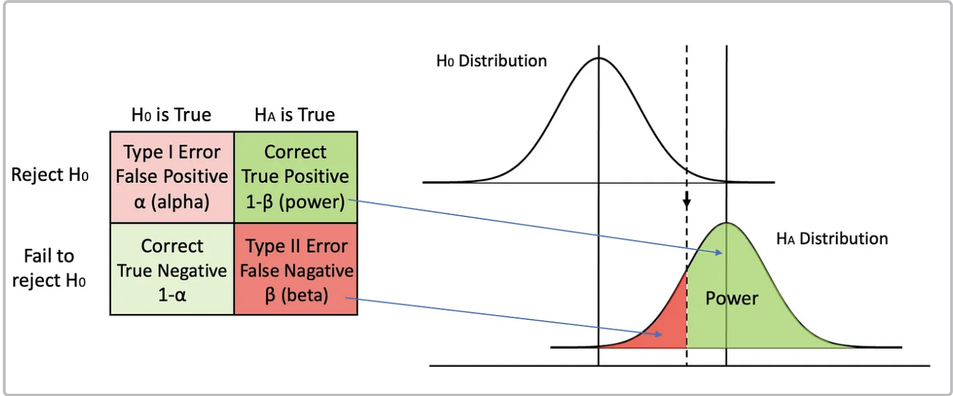
The flip side of significance: Statistical power

Don’t forget to give yourself a fighting chance to find the effect you are looking for!

Applications

Application readings

Let’s level-set people’s familiarity with these pieces.

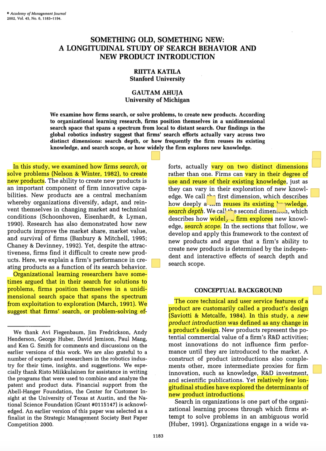
Katila, R., & Ahuja, G. 2002. Something Old, Something New: A Longitudinal Study of Search Behavior and New Product Introduction. Academy of Management Journal, 45(6), 1183-1194.
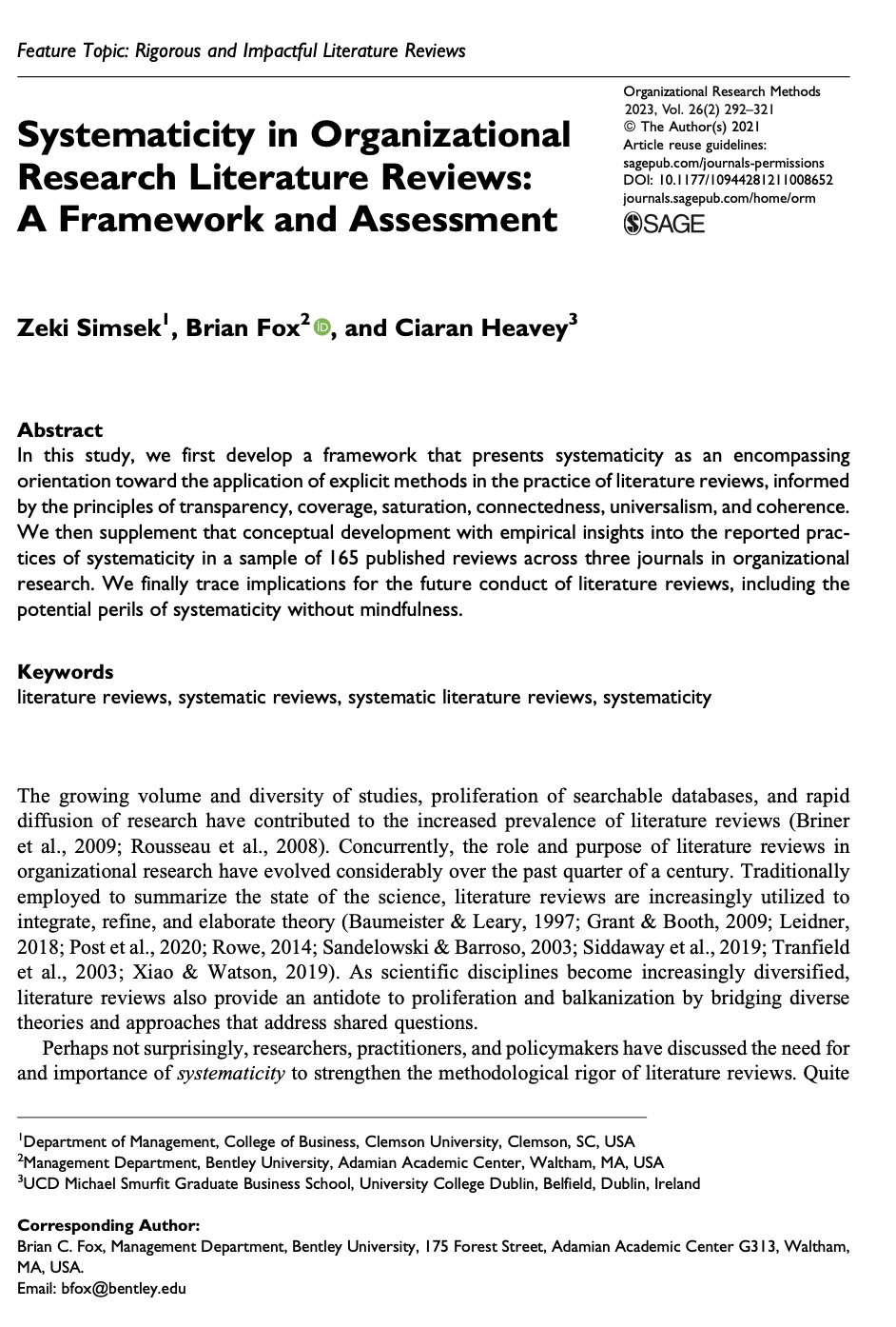
Simsek, Z., Fox, B., & Heavey, C. 2021. Systematicity in Organizational Research Literature Reviews: A Framework and Assessment. Organizational Research Methods, 109442812110086.

Katila and Ahuja (2002)

What was this paper about?
What were the findings?
What was the method?
What makes sense? What was confusing?

Simsek Fox and Heavey (2021)

What was this paper about?
What were the findings?
What was the method?
What makes sense? What was confusing?

Break

Replication Presentation

Replication: Simsek, Z., Fox, B., & Heavey, C. 2021. Systematicity in Organizational Research Literature Reviews: A Framework and Assessment. Organizational Research Methods, 109442812110086.

Skills corner

Class walkthrough in R

Our “skills corner” for the rest of the semester is embedded in two parts of the class:
- The “how to” discussion in the first hour, talking about the general process
- The “workshop” now where we apply these ideas in the context of R
- Let’s fire up R and see how to execute

General discussion

Preparation for next class

Next class

Concept check 2 will available this evening - please complete it before next class.

Next class

Techniques II: Moderation

Dawson, J. F. 2014. Moderation in Management Research: What, Why, When, and How. Journal of Business and Psychology, 29(1), 1-19.
Hitt, M. A., Beamish, P. W., Jackson, S. E., & Mathieu, J. E. 2007. Building Theoretical and Empirical Bridges Across Levels: Multilevel Research in Management. Academy of Management Journal, 50(6), 1385-1399.

Next class

Techniques II: Moderation

Applications:

Replication: Heavey, C., Simsek, Z., & Fox, B. C. 2015. Managerial Social Networks and Ambidexterity of SMEs: The Moderating Role of a Proactive Commitment to Innovation. Human Resource Management, 54(S1).
Wolfson, M. A., & Mathieu, J. E. 2018. Sprinting to the finish: Toward a theory of Human Capital Resource Complementarity. J Appl Psychol, 103(11), 1165-1180.

References

Angrist, J. D., and J. S Pischke. 2008. Mostly Harmless Econometrics: An Empiricist’s Companion. Princeton, NJ: Princeton University Press.

Carlson, Kevin D., and Jinpei Wu. 2012. “The Illusion of Statistical Control.” Organizational Research Methods 15 (3): 413–35.

Fox, Brian C., Zeki Simsek, and Ciaran Heavey. 2022. “Top Management Team Experiential Variety, Competitive Repertoires, and Firm Performance: Examining the Law of Requisite Variety in the 3D Printing Industry (1986–2017).” Academy of Management Journal 65 (2): 545–76.

———. 2023. “Venture Team Membership Dynamics and New Venture Innovation.” Strategic Entrepreneurship Journal.

Greene, William H. 2012. “Econometric Analysis.”

Kennedy, Peter. 2008. A Guide to Econometrics. Malden, MA: Blackwell.